Summary: Grafana Tempo is an open-source distributed tracing backend that uses object storage to cut costs, scale effortlessly, and simplify debugging across microservices.
If you have ever spent hours trying to track down a bug that started in one microservice and rippled through five others before causing a failure, you understand the problem that distributed tracing solves. When a single user request passes through a web server, an authentication service, a payment processor, and a database, all potentially running on separate machines, traditional logging quickly becomes insufficient. You need a way to follow that request through every hop and see exactly where things went wrong.
Grafana Tempo is an open-source, high-volume distributed tracing backend built to do exactly that. It stores and retrieves traces efficiently, at massive scale, and at a fraction of the cost of traditional tracing systems.
This guide explains what Grafana Tempo is, how its architecture works, what sets it apart from tools like Jaeger and Zipkin, and how to get started using it in your observability stack.
Key Takeaways
- Simplify distributed tracing at scale by using Grafana Tempo’s object storage architecture to eliminate costly index databases.
- Query billions of spans instantly with TraceQL to pinpoint slow requests, errors, and service bottlenecks.
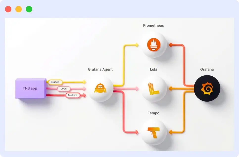
- Connect Tempo traces with Prometheus metrics and Loki logs for complete incident visibility in one workflow.
- Cut mean time to resolution with Middleware by automatically correlating traces, logs, and infrastructure metrics without extra configuration.
Grafana is just one part of the observability stack. See how it compares with other tools.
What is Grafana Tempo?
Grafana Tempo is an open-source distributed tracing backend developed by Grafana Labs. It ingests, stores, and queries trace data at high volume without the operational complexity that traditional tracing systems require.
Grafana Labs created the project to address a specific problem: most tracing backends require you to maintain expensive, index-heavy databases (like Elasticsearch or Cassandra) to make traces searchable. This works at a small scale but becomes prohibitively expensive and difficult to manage as the trace volume grows.
Tempo takes a fundamentally different approach by writing traces directly to object storage services such as Amazon S3, Google Cloud Storage, or Azure Blob Storage, skipping the indexing layer entirely.
The result is a tracing backend that is simpler to operate, dramatically cheaper at scale, and capable of handling millions of spans per second.
Key fact: Grafana Tempo requires only object storage to operate. There are no index databases to provision, tune, or maintain.
Traces and Spans
Before going further, it helps to understand the two core concepts that underpin all distributed tracing:
- A span represents a single unit of work within a request. For example, one span might represent a call to a database, another might represent an HTTP request to an external API, and another might represent processing time within a specific function.
- A trace is the complete picture of a single request as it travels through your system. Tempo assembles it from all individual spans that share the same trace ID. A trace shows you the full timeline of a request, which services it touched, in what order, and how long each step took.
When a user clicks a button in your application and that action triggers a chain of microservice calls, Tempo collects all of the spans from every service involved and assembles them into a single trace. You can then view that trace as a flame graph or waterfall chart and see, at a glance, exactly where time went and whether any errors occurred.
How does Grafana Tempo Work?
Understanding Tempo’s architecture explains both its strengths and its design trade-offs. Several distinct components make up the system, each handling a specific part of the tracing pipeline.
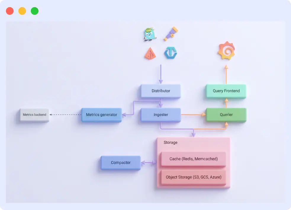
The Core Components
Distributor
The distributor is the entry point for all incoming trace data. It receives spans from your instrumented applications using supported ingestion protocols (OpenTelemetry, Jaeger, or Zipkin), validates them, and forwards them to the appropriate ingester based on the trace ID. The distributor is stateless and horizontally scalable; you can run as many distributors as your ingest volume requires.
Ingester
The ingester receives spans from the distributor and temporarily stores them in memory. It batches incoming spans by trace ID and periodically flushes complete or partially complete traces to the backend object storage. The ingester also serves queries for very recent traces it has not yet flushed to storage.
Compactor
The compactor runs in the background and merges smaller trace blocks in object storage into larger, more efficient blocks. This process reduces storage costs and improves query performance over time by organizing data into a faster-to-scan structure.
Query Frontend and Querier
When you search for a trace, the query frontend receives your request, breaks it into sub-queries, and distributes them across multiple querier instances. The queriers retrieve trace blocks from object storage, search for matching traces, and return the results. The query frontend then assembles the final response. This parallelized approach enables Tempo to efficiently search large volumes of trace data.
Object Storage Backend
All trace data ultimately lives in object storage. Tempo supports Amazon S3, Google Cloud Storage, Azure Blob Storage, and local filesystem storage (for development). Object storage is the foundation of Tempo’s cost advantage. It is significantly cheaper per gigabyte than database storage, and it scales without capacity planning.
TraceQL: Querying Your Traces
Tempo includes TraceQL, a purpose-built query language for searching and filtering trace data. If you are familiar with SQL or PromQL, the syntax will feel intuitive, but instead of querying rows in a database or time-series metrics, you are querying spans and traces.
TraceQL lets you filter traces by service name, span duration, status codes, HTTP methods, custom attributes, and more. You can combine conditions to find exactly the traces you need, even across billions of spans.
Here are a few examples of what TraceQL queries look like:
All traces flagged with an error status
{ status = error }Find traces where a specific service took longer than 2 seconds
{ .service.name = "checkout" && duration > 2s }Find traces that passed through both the auth service and the payment service
{ .service.name = "auth" } && { .service.name = "payment" }TraceQL is also the foundation for Tempo’s streaming search, which allows queries to return results incrementally rather than waiting for the entire scan to complete, a significant usability improvement at scale.
Grafana Tempo vs. Jaeger and Zipkin
Jaeger and Zipkin are the two most widely used open-source tracing backends before Tempo’s introduction. Both are mature, well-supported projects, but they share an architectural pattern that Tempo deliberately avoids: index-based storage.
In Jaeger and Zipkin, each incoming trace is indexed with service names, operation names, tags, and timestamps, and the resulting index is stored in a searchable repository (typically Cassandra or Elasticsearch). This makes ad-hoc queries fast and flexible, but it comes with significant trade-offs at scale.
Tempo’s approach eliminates the index entirely, trading some query flexibility for major gains in cost and operational simplicity. The comparison below summarizes the key differences:
| Feature | Grafana Tempo | Jaeger / Zipkin |
|---|---|---|
| Storage | Object storage (S3, GCS, Azure Blob) | Cassandra, Elasticsearch, or in-memory |
| Indexing | No indexing (writes directly to storage) | Full index of every trace |
| Cost at scale | Very low (object storage is cheap) | High (index databases are expensive) |
| Operational complexity | Low (no index tuning required) | High (requires database management) |
| Query language | TraceQL (powerful, purpose-built) | UI-based or basic query filters |
| Ingestion protocols | OTLP, Jaeger, Zipkin | Jaeger or Zipkin only (respectively) |
| Horizontal scalability | Unlimited (add object storage) | Limited by database capacity |
The practical implication is that Tempo is not always the right choice for every use case.
If your team runs a small-scale deployment and needs highly flexible, ad-hoc tag-based searches without writing TraceQL, Jaeger may be a better fit.
But for teams running distributed systems at significant scale, where storage costs and operational overhead are real concerns, Tempo’s architecture offers compelling advantages.
Core Features of Grafana Tempo
Grafana Tempo isn’t just another tracing tool; it’s built from the ground up to solve real-world problems at scale. Let’s explore what makes it stand out.
Horizontal Scalability
Each component in Tempo’s architecture scales independently. If your ingest volume spikes, you add more distributors and ingesters. If query load increases, you add more queriers.
There is no central bottleneck, no resharding process, and no downtime required. In practice, Tempo deployments handle millions of spans per second without architectural changes; you simply provision more instances.
Cost Efficiency
The cost advantage of object-storage-only tracing is substantial. Storing 1 TB in Elasticsearch or Cassandra can cost an order of magnitude more than storing the same 1 TB in Amazon S3 or Google Cloud Storage. For organizations generating high trace volumes, this difference translates directly into significant monthly savings.
Tempo also gives you control over retention periods, allowing you to keep traces for 30 days, 90 days, or longer based on your needs and budget.
Multi-Tenancy
Tempo supports multi-tenancy natively, allowing multiple teams or products to share a single Tempo deployment while keeping their trace data isolated. Each tenant gets its own storage namespace, and you can configure per-tenant limits on ingest rate, trace length, and retention.
This makes Tempo practical for platform teams that want to run a centralized observability infrastructure for multiple engineering teams.
Exemplars for Cross-Signal Correlation
Exemplars are data points embedded in Prometheus metrics that carry a trace ID. When Tempo is connected to Grafana alongside Prometheus and Loki, exemplars create direct links between your metric dashboards and your traces. You can see a latency spike in a Prometheus chart and click directly into the trace that caused it, no manual searching, no copy-pasting trace IDs. This cross-signal workflow significantly reduces the time it takes to move from alert to root cause.
Protocol Flexibility
Tempo accepts traces in all three major formats: OpenTelemetry (OTLP), Jaeger, and Zipkin. This means you can adopt Tempo without replacing your existing instrumentation. Teams already using Jaeger agents can point them at Tempo by changing a configuration. Teams adopting OpenTelemetry from scratch will find first-class support throughout.
Setup and Deployment of Grafana Tempo
Tempo can be deployed in two ways: as a self-hosted system on your own infrastructure, or as a fully managed service through Grafana Cloud. Both options are covered below.
Option 1: Grafana Cloud Tempo (Managed)
Grafana Cloud Tempo handles all infrastructure, storage, and upgrades for you. To get started, sign up at grafana.com, navigate to your Grafana Cloud portal, and go to the Tempo section to retrieve your endpoint and credentials.
Configure your OpenTelemetry Collector to send traces to Grafana Cloud:
# OpenTelemetry Collector configuration for Grafana Cloud Tempo
exporters:
  otlp:
    endpoint: "tempo-<your-instance>.grafana.net:443"
    headers:
      authorization: "Basic <your-base64-encoded-credentials>"

service:
  pipelines:
    traces:
      exporters: [otlp]
Replace <your-instance> With your Grafana Cloud instance name, encode your credentials as instanceID:api_token in base64. Your applications are now sending traces to the cloud with no servers to maintain.
Option 2: Self-Hosted Tempo on Kubernetes
Self-hosting gives you full control over your Tempo deployment. The recommended approach is to use Grafana’s official Helm chart.
Step 1: Install Tempo with Helm
# Add the Grafana Helm repository
helm repo add grafana https://grafana.github.io/helm-charts

# Update your Helm repositories
helm repo update

# Install Tempo with default configuration
helm install tempo grafana/tempo-distributed -n tempo --create-namespace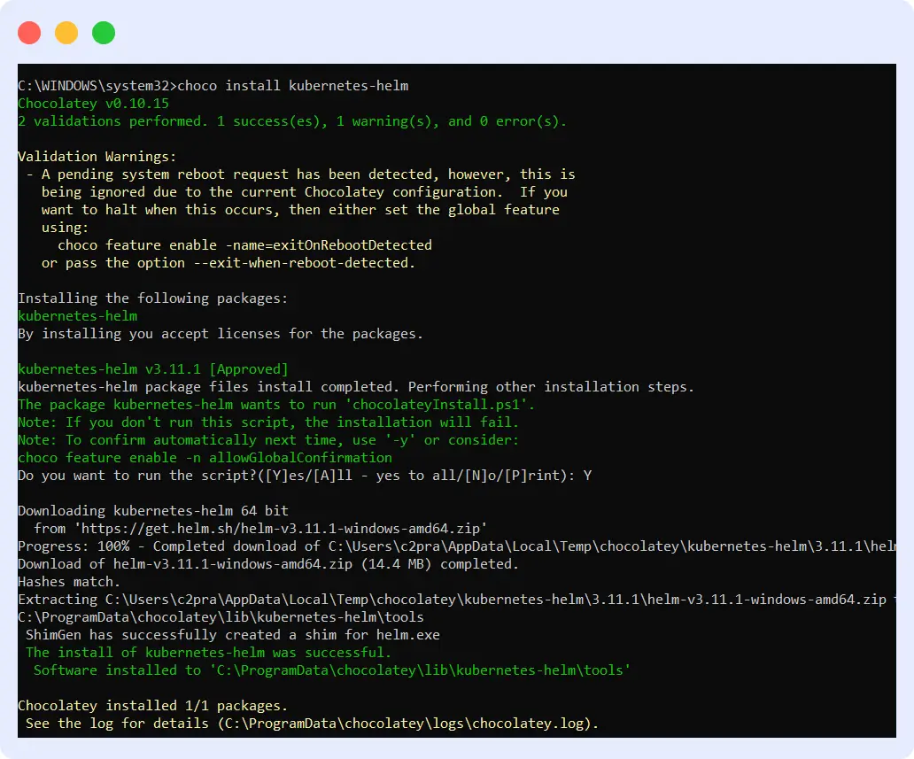
Within minutes, you’ll have the Grafana Tempo architecture deployed and running. You can verify the installation with:
# Check if all Tempo pods are running
kubectl get pods -n tempo
Step 2: Configure Your Object Storage
Next, set up your Grafana Tempo object storage backend. Whether you’re using S3, Google Cloud Storage, or Azure Blob, you’ll need to provide your storage credentials and bucket details in Tempo’s configuration file. This is where all your traces will live. For this, you need to create a configuration file called tempo-values.yaml:
# tempo-values.yaml
tempo:
  storage:
    trace:
      backend: s3
      s3:
        bucket: your-tempo-traces-bucket
        endpoint: s3.amazonaws.com
        access_key: YOUR_ACCESS_KEY
        secret_key: YOUR_SECRET_KEY
        insecure: false

  retention: 720h  # 30 days retention
Now upgrade your Tempo installation with this configuration:
# Apply your custom storage configuration
helm upgrade tempo grafana/tempo-distributed -n tempo -f tempo-values.yaml
Whether you’re using S3, Google Cloud Storage (use backend: gcs), or Azure Blob (use backend: azure), just update the backend type and credentials accordingly. This is where all your traces will live.
Step 3: Connect Tempo to Grafana
Add Tempo as a data source in Grafana by creating a data source configuration file:
# grafana-datasource.yaml
apiVersion: 1

datasources:
  - name: Tempo
    type: tempo
    access: proxy
    url: http://tempo-query-frontend.tempo:3100
    uid: tempo
    editable: true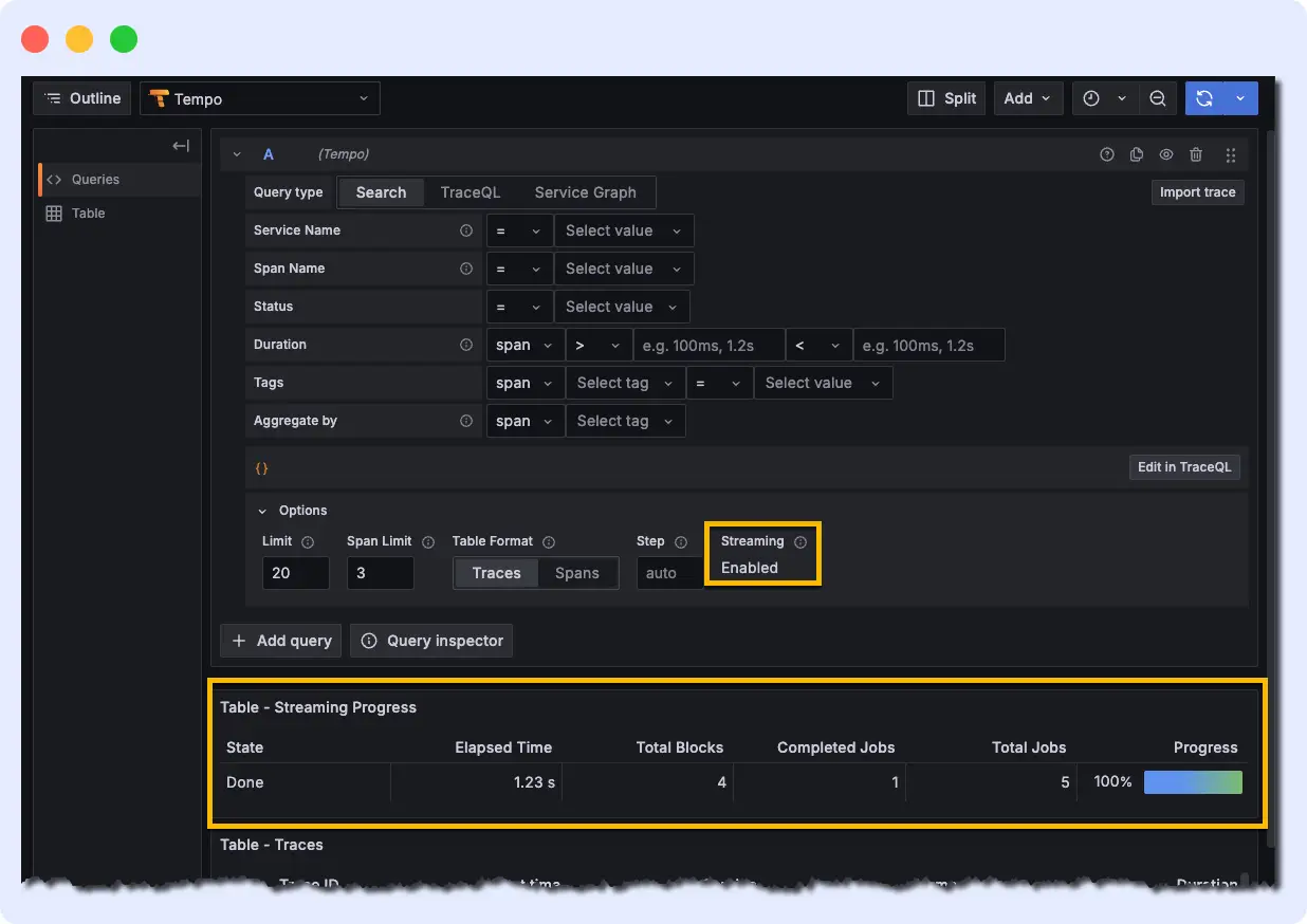
Apply this via Grafana’s UI (Configuration > Data Sources > Add data source > Tempo) or by passing the file to your Grafana deployment. Once connected, you can query traces using TraceQL directly from Grafana’s Explore view.
Now you can query traces using TraceQL and see your distributed tracing data come to life in beautiful dashboards.
That’s it! You’re now running a production-ready tracing backend. Start sending traces from your applications using OpenTelemetry, Jaeger, or Zipkin protocols, and watch as Tempo captures every request flowing through your system.
Integrating Tempo into Your Observability Stack
Let’s see how Tempo transforms from a standalone tool into the backbone of your debugging workflow.
Exploring Traces in Grafana
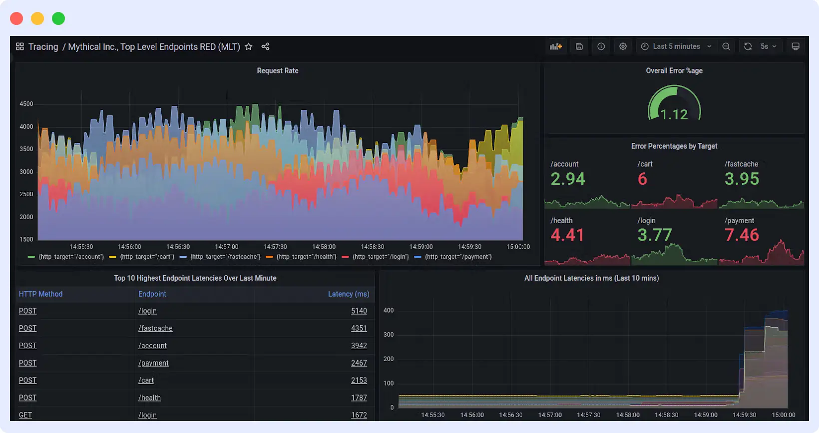
With Tempo connected as a data source, Grafana’s Explore view becomes your primary interface for trace analysis. Select Tempo as the data source, write a TraceQL query or search by trace ID, and Grafana renders the trace as an interactive flame graph or waterfall chart. Each span is clickable and shows its duration, attributes, and any associated logs or errors.
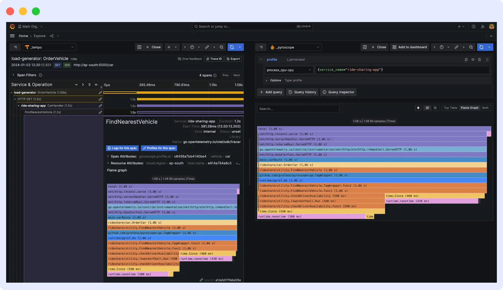
You’ll see beautiful visualizations showing how requests flow through your services, where time is spent, and which operations are slowing things down. Every span is clickable, every timing is clear, and you can drill down into any part of your system’s behavior.
Connecting the Dots: Metrics, Traces, and Logs
Tempo becomes most powerful when used alongside Prometheus (for metrics) and Loki (for logs). The connection among these three systems is mediated by exemplar reference points that embed a trace ID in a Prometheus metric data point.
When you configure your applications to emit exemplars, a latency spike in a Prometheus dashboard becomes a clickable link to the exact trace that caused it.
From that trace, you can jump to the Loki logs from the same request using the trace ID as a shared identifier. This three-way connection metric, when traced in the logs, provides a complete picture of any incident without requiring manual correlation across systems.
Example: Diagnosing a Latency Spike
Here is a concrete example of this workflow in practice. Your Prometheus dashboard shows a 95th-percentile latency spike in your checkout service. You click the exemplar on the chart, which opens the corresponding trace in Tempo.
The trace shows that the payment API call, which normally takes 200ms, is now taking 5 seconds, and the span has an error attribute pointing to a database timeout.
You follow the trace ID into Loki and see the database error logs from that exact request window. In under two minutes, you have gone from a latency alert to a confirmed root cause, without writing a single ad-hoc query or manually grepping log files.
Expanding Grafana Tempo with Unified Observability
Distributed tracing gives you a detailed view of individual requests as they move through your system. But traces alone do not tell the complete story of an incident.
A slow trace might be caused by a saturated CPU on a specific pod, a memory leak that spiked two minutes earlier, or a flood of error logs in a downstream service.
To diagnose issues quickly, you need traces, metrics, and logs to be connected rather than stored in separate silos that require manual correlation.
This is where Middleware extends what Grafana Tempo provides. Middleware works alongside your existing Tempo deployment, whether self-hosted or on Grafana Cloud, and automatically correlates your trace data with logs and infrastructure metrics.
You do not need to change how Tempo is configured or how your applications are instrumented. Middleware connects the dots between what happened (traces), what was logged (logs), and what the numbers show (metrics), giving your engineering team unified context in a single interface.
How the Integration Works
Middleware integrates with Grafana Tempo through the OpenTelemetry Collector. Raw trace data flows from your applications into Tempo as normal.
Simultaneously, Middleware ingests the same telemetry and uses it to automatically build cross-signal context. It injects trace_id and span_id metadata directly into application logs, so every log entry is indexed against the specific request that generated it.
This eliminates the need to manually configure log correlation or write custom middleware to propagate trace context through your logging stack.
Beyond log correlation, Middleware maps individual trace spans to the underlying infrastructure metrics of the container or pod that executed them. When a span shows a latency spike, Middleware can surface whether the relevant container was experiencing CPU saturation, memory pressure, or network throttling at the same moment.
This span to infrastructure mapping is what turns a slow trace into an actionable root cause. Instead of knowing that a service was slow, you know exactly which resource constraint caused it.
Reducing MTTR in Practice
The practical effect of this integration is a faster debugging workflow. In a standard Grafana Tempo setup, diagnosing an incident involves querying Tempo for relevant traces, noting the trace ID, switching to Loki to search for related logs, and separately checking your metrics dashboards for infrastructure signals. Each context switch adds time and cognitive load.
With Middleware, the workflow collapses into a single interface. An engineer notices a service anomaly, clicks on it, and immediately sees the correlated distributed trace, the relevant log entries from that request, and the infrastructure metrics from the pod that served it, all in context, all without writing a TraceQL query or switching between tools.
This reduction in friction directly reduces mean time to resolution (MTTR), particularly for complex incidents that span multiple services and infrastructure layers.
Middleware works alongside Grafana Tempo without requiring any changes to your existing Tempo configuration, instrumentation, or storage setup. It ingests the same OpenTelemetry data and uses it to build cross-signal connections that Tempo alone cannot provide.
What This Means for Your Observability Stack
Grafana Tempo handles the hard problem of storing and querying trace data at scale. Middleware takes that trace data and connects it to everything else happening in your system.
The two tools are complementary: Tempo gives you the raw tracing foundation, and Middleware builds the observability layer on top of it that makes traces operationally useful during an incident.
For teams already running Grafana, Prometheus, and Loki alongside Tempo, Middleware extends this existing stack rather than replacing it. It provides enhanced visualizations that surface patterns and anomalies that are easy to miss in standard dashboards, and its AI-driven insights automatically flag unusual trace behavior, identifying increases in error rates, latency regressions, and throughput drops without requiring engineers to write and maintain alert rules for every failure mode.
If you want to see how Middleware fits into your existing Tempo deployment, you can request a demo.
Best Practices for Running Grafana Tempo
You’ve got Grafana Tempo up and running – awesome! Now let’s make sure you’re using it like a pro. These battle-tested tips will save you headaches, money, and debugging time down the road.
Start with Critical Services
Instrument your most important services first, those handling authentication, payments, or core business logic. Attempting to instrument everything at once creates unnecessary complexity and makes it harder to validate that your tracing setup is working correctly.
Once you have confirmed that traces are flowing and the data is useful, expand incrementally to other services.
Maintain Consistent Trace IDs Across Signals
For the metrics-to-traces-to-logs workflow to function correctly, the same trace ID must appear in your traces, your metric exemplars, and your log entries.
This requires consistent instrumentation across your services and careful configuration of your logging libraries to inject the current trace context into every log line. Without this consistency, you lose the ability to correlate signals across systems and must fall back to manual debugging.
Set and Monitor Retention Policies
Object storage costs accumulate over time. Define a clear retention policy before you go to production. 30 days is a reasonable default for most teams, with longer retention for business-critical services. Monitor your storage bucket size regularly and adjust your sampling rates or retention windows if costs start to exceed expectations.
Use Head Sampling to Manage Volume
Not every trace needs to be stored. For high-traffic services, head-based sampling, making a keep-or-discard decision at the start of a trace, lets you capture a representative percentage of traffic while controlling storage costs.
Tempo integrates with the OpenTelemetry Collector’s probabilistic sampler for this purpose. A common approach is to capture error traces while sampling only a small percentage of successful ones.
Automate Deployments Through CI/CD
Configuration changes to Tempo, updated retention policies, new storage credentials, and version upgrades should be deployed through your standard CI/CD pipeline rather than applied manually.
Manual changes to production observability infrastructure are a common source of outages and configuration drift. Treat your Tempo configuration as code and apply the same review and deployment standards you use for your application code.
Plan for Cloud Storage Costs
Before deploying Tempo in production, estimate your expected trace volume and calculate the monthly object storage cost at your intended retention period.
Factor in egress costs if your application and storage are in different regions, and consider using S3 Intelligent-Tiering or equivalent features for older trace data. A modest investment in cost planning upfront prevents unpleasant billing surprises at scale.
Conclusion
Grafana Tempo solves a real problem: distributed tracing at scale has historically been expensive and operationally complex, which led many teams to skip it or adopt minimal tracing coverage.
By replacing index-based storage with object storage and providing TraceQL as a capable query interface, Tempo makes comprehensive distributed tracing accessible to teams of all sizes.
Its architecture scales horizontally without bottlenecks, its storage costs are a fraction of traditional tracing systems, and its integration with Grafana, Prometheus, and Loki creates a coherent observability stack where signals are connected rather than siloed.
To go further, the following resources are a good starting point:
- Official Grafana Tempo documentation, Tempo Helm chart, TraceQL reference, Grafana community forums.